1. Exploring the Brown Dwarf Synthetic Dataset
In the following steps, you will:
Load the brown dwarf synthetic spectra used to train the ML models
Check the variables and parameters in the dataset
Visualize them for few cases
Before going through this tutorial, make sure you have installed TelescopeML (Install through Git) successfully as discussed in this installation link.
Note: The latest version is located on GitHub, so please follow the instructions provided in the “Method 1: Install through Git (Recommended)” section of the link to install the package.
In a nutshell:
[1] You have already:
Created the TelescopeML_project directory.
Downloaded the reference_data from this link.
Cloned TelescopeML using
git clone https://github.com/EhsanGharibNezhad/TelescopeML.git.
[2] The trained ML models, datasets, figures, and tutorials (or notebooks) are now all in your TelescopeML_project/reference_data directory.
[3] The path is defined to your reference_data. Confirm it by os.getenv("TelescopeML_reference_data"), but if you encounter an error, simply hard code it by defining the path as __reference_data_path__.
[4] Lastly, you should be able to execute import TelescopeML without any issues!
Happy TelescopeMLing! ;)
[1]:
# Let's first import libraries we need in this tutorial!
from TelescopeML.StatVisAnalyzer import *
No Bottleneck unit testing available.
1.1 Load the Synthetic spectra
We computed a low-resolution spectrum (\(R\)=200) utilizing atmopshric brown dwarfs grid model, Sonora-Bobcat for spectral range $:nbsphinx-math:sim`$0.9-2.4 :math:mu m`. An open-source atmospheric radiative transfer Python package, PICASO was employed for generating these datasets. This dataset encompass 30,888 synthetic spectra (or instances or rows).
Each spectrum has 104 wavelengths (i.e., 0.897, 0.906, …, 2.512 μm) and 4 output atmospheric parameters:
gravity (log g)
temperature (Teff)
carbon-to-oxygen ratio (C/O)
metallicity ([M/H])
[2]:
import os

__reference_data_path__ = os.getenv("TelescopeML_reference_data")
__reference_data_path__


# Note: insert the directory of the reference_data if you get an error reading the reference data!!!
# __reference_data_path__ = 'INSERT_DIRECTORY_OF_reference_data'
[2]:
'/Users/egharibn/RESEARCH/ml/projects/TelescopeML_project/reference_data/'
Load the dataset and check few instances
[3]:
train_BD = pd.read_csv(os.path.join(__reference_data_path__,
                                    'training_datasets',
                                    'browndwarf_R100_v4_newWL_v3.csv.bz2'), compression='bz2')
train_BD
[3]:
| gravity | temperature | c_o_ratio | metallicity | 2.512 | 2.487 | 2.462 | 2.438 | 2.413 | 2.389 | ... | 0.981 | 0.971 | 0.962 | 0.952 | 0.943 | 0.933 | 0.924 | 0.915 | 0.906 | 0.897 | |
|---|---|---|---|---|---|---|---|---|---|---|---|---|---|---|---|---|---|---|---|---|---|
| 0 | 5.00 | 1100 | 0.25 | -1.0 | 9.103045e-08 | 1.181658e-07 | 1.307868e-07 | 1.269229e-07 | 1.159179e-07 | 8.925110e-08 | ... | 1.257751e-07 | 9.640859e-08 | 7.612550e-08 | 6.901364e-08 | 6.247359e-08 | 4.112384e-08 | 5.127995e-08 | 4.897355e-08 | 4.087795e-08 | 2.791689e-08 |
| 1 | 5.00 | 1100 | 0.25 | -0.7 | 9.103045e-08 | 1.181658e-07 | 1.307868e-07 | 1.269229e-07 | 1.159179e-07 | 8.925110e-08 | ... | 1.257751e-07 | 9.640859e-08 | 7.612550e-08 | 6.901364e-08 | 6.247359e-08 | 4.112384e-08 | 5.127995e-08 | 4.897355e-08 | 4.087795e-08 | 2.791689e-08 |
| 2 | 5.00 | 1100 | 0.25 | -0.5 | 9.103045e-08 | 1.181658e-07 | 1.307868e-07 | 1.269229e-07 | 1.159179e-07 | 8.925110e-08 | ... | 1.257751e-07 | 9.640859e-08 | 7.612550e-08 | 6.901364e-08 | 6.247359e-08 | 4.112384e-08 | 5.127995e-08 | 4.897355e-08 | 4.087795e-08 | 2.791689e-08 |
| 3 | 5.00 | 1100 | 0.25 | -0.3 | 9.103045e-08 | 1.181658e-07 | 1.307868e-07 | 1.269229e-07 | 1.159179e-07 | 8.925110e-08 | ... | 1.257751e-07 | 9.640859e-08 | 7.612550e-08 | 6.901364e-08 | 6.247359e-08 | 4.112384e-08 | 5.127995e-08 | 4.897355e-08 | 4.087795e-08 | 2.791689e-08 |
| 4 | 5.00 | 1100 | 0.25 | 0.0 | 9.103045e-08 | 1.181658e-07 | 1.307868e-07 | 1.269229e-07 | 1.159179e-07 | 8.925110e-08 | ... | 1.257751e-07 | 9.640859e-08 | 7.612550e-08 | 6.901364e-08 | 6.247359e-08 | 4.112384e-08 | 5.127995e-08 | 4.897355e-08 | 4.087795e-08 | 2.791689e-08 |
| ... | ... | ... | ... | ... | ... | ... | ... | ... | ... | ... | ... | ... | ... | ... | ... | ... | ... | ... | ... | ... | ... |
| 30883 | 3.25 | 1000 | 2.50 | 0.7 | 1.533414e-08 | 1.244438e-08 | 7.703017e-09 | 5.262130e-09 | 4.671165e-09 | 3.026652e-09 | ... | 2.064408e-08 | 1.919290e-08 | 1.685050e-08 | 1.772466e-08 | 1.726968e-08 | 1.341722e-08 | 1.365819e-08 | 8.811601e-09 | 4.752807e-09 | 2.206752e-09 |
| 30884 | 3.25 | 1000 | 2.50 | 1.0 | 6.942763e-09 | 5.536744e-09 | 3.501408e-09 | 2.445445e-09 | 2.168689e-09 | 1.477159e-09 | ... | 4.353813e-09 | 4.401064e-09 | 4.029425e-09 | 4.482797e-09 | 4.647158e-09 | 3.722947e-09 | 3.825720e-09 | 1.921753e-09 | 8.112957e-10 | 3.211086e-10 |
| 30885 | 3.25 | 1000 | 2.50 | 1.3 | 3.758895e-09 | 2.988295e-09 | 1.968653e-09 | 1.417744e-09 | 1.260679e-09 | 9.059680e-10 | ... | 1.546743e-09 | 1.698977e-09 | 1.577032e-09 | 1.813035e-09 | 1.915084e-09 | 1.497190e-09 | 1.512469e-09 | 5.734859e-10 | 1.823897e-10 | 6.218672e-11 |
| 30886 | 3.25 | 1000 | 2.50 | 1.7 | 3.150169e-09 | 2.503614e-09 | 1.672564e-09 | 1.218379e-09 | 1.085002e-09 | 7.942492e-10 | ... | 1.332727e-09 | 1.481450e-09 | 1.346700e-09 | 1.538485e-09 | 1.608156e-09 | 1.223594e-09 | 1.254078e-09 | 4.561500e-10 | 1.370389e-10 | 4.616465e-11 |
| 30887 | 3.25 | 1000 | 2.50 | 2.0 | 2.665630e-09 | 2.117952e-09 | 1.434730e-09 | 1.055994e-09 | 9.418247e-10 | 7.020869e-10 | ... | 1.533098e-09 | 1.647372e-09 | 1.385020e-09 | 1.517044e-09 | 1.524311e-09 | 1.096679e-09 | 1.209663e-09 | 4.837326e-10 | 1.534210e-10 | 5.612844e-11 |
30888 rows × 108 columns
1.2 Check atmospheric parameters
gravity (log g)
temperature (Teff)
carbon-to-oxygen ratio (C/O)
metallicity ([M/H])
[4]:
output_names = ['gravity', 'temperature', 'c_o_ratio', 'metallicity']
train_BD[output_names].head()
[4]:
| gravity | temperature | c_o_ratio | metallicity | |
|---|---|---|---|---|
| 0 | 5.0 | 1100 | 0.25 | -1.0 |
| 1 | 5.0 | 1100 | 0.25 | -0.7 |
| 2 | 5.0 | 1100 | 0.25 | -0.5 |
| 3 | 5.0 | 1100 | 0.25 | -0.3 |
| 4 | 5.0 | 1100 | 0.25 | 0.0 |
1.3 Check the synthetic spectra
[5]:
wavelength_names = [item for item in train_BD.columns.to_list() if item not in output_names]
wavelength_names[:5]
[5]:
['2.512', '2.487', '2.462', '2.438', '2.413']
[6]:
wavelength_values = [float(item) for item in wavelength_names]
wavelength_values[:10]
[6]:
[2.512, 2.487, 2.462, 2.438, 2.413, 2.389, 2.366, 2.342, 2.319, 2.296]
1.4 Visualize the Brown Dwarf spectra for different parameters
1.4.1 Effective Temperature
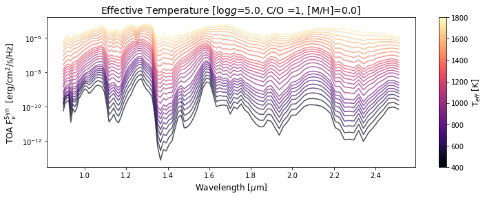
Plot the brown dwarf datasets for \(T_{\rm eff}\)= 400-1800K while other paremeters are constnat (logg=5, C/O=1, [M/H]=0)
[7]:
# Define the filter bounds
filter_bounds = {'gravity': (5.,5),
                 'c_o_ratio' : (1,1),
                 'metallicity' : (0.0,0.0),
                 'temperature': (400, 1800)}

# Call the function to filter the dataset
plot_filtered_spectra(
                    dataset = train_BD,
                    filter_bounds = filter_bounds,
                    feature_to_plot = 'temperature',
                    title_label = '[log$g$='+str(filter_bounds['gravity'][0])+
                                  ', C/O ='+str(filter_bounds['c_o_ratio'][0])+
                                  ', [M/H]='+str(filter_bounds['metallicity'][0])+']',
                    wl_synthetic = wavelength_values,
                    output_names = output_names,
                    __reference_data__ = __reference_data_path__,
                    __save_plots__=True,
                    )

1.4.2 Gravity
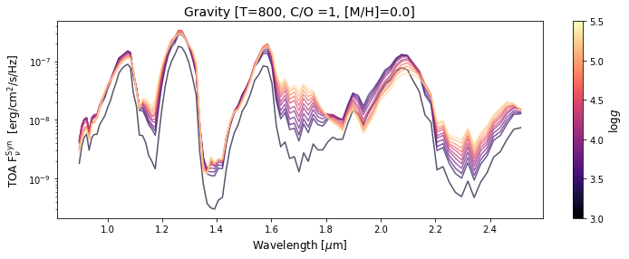
Plot the brown dwarf datasets for log\(g\)= 3-5.5 while other paremeters are constnat (\(T_{eff}\)=800, C/O=1, [M/E]=0)
[8]:
# Define the filter bounds
filter_bounds = {'gravity': (3,5.5),
                 'c_o_ratio' : (1,1),
                 'metallicity' : (0.0,0.0),
                 'temperature': (800, 800)}

# Call the function to filter the dataset
plot_filtered_spectra(
                        dataset = train_BD,
                        filter_bounds = filter_bounds,
                        feature_to_plot = 'gravity',
                        title_label =   '[T='+str(filter_bounds['temperature'][0])+
                                        ', C/O ='+str(filter_bounds['c_o_ratio'][0])+
                                        ', [M/H]='+str(filter_bounds['metallicity'][0])+']',
                        wl_synthetic = wavelength_values,
                        output_names = output_names,
                        __reference_data__ = __reference_data_path__,
                        __save_plots__=True,
                    )

1.4.3 Carbon-to-Oxygen ratio
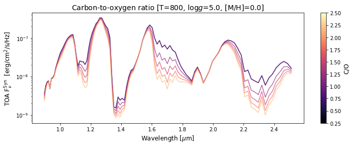
Plot the brown dwarf datasets for C/O= 0.25-2.5 while other paremeters are constnat (Teff=800, log g=5.0, [M/H]=0)
[9]:
# Define the filter bounds
filter_bounds = {'gravity': (5.,5),
                 'c_o_ratio' : (0.25,2.5),
                 'metallicity' : (0.0,0.0),
                 'temperature': (800, 800)}


# Call the function to filter the dataset
plot_filtered_spectra(
                        dataset = train_BD,
                        filter_bounds = filter_bounds,
                        feature_to_plot = 'c_o_ratio',
                        title_label = '[T='+str(filter_bounds['temperature'][0])+
                                    ', log$g$='+str(filter_bounds['gravity'][0])+
                                    ', [M/H]='+str(filter_bounds['metallicity'][0])+']',
                        wl_synthetic = wavelength_values,
                        output_names = output_names,
                        __reference_data__ = __reference_data_path__,
                        __save_plots__=True,
                    )

1.4.4 Metallicity
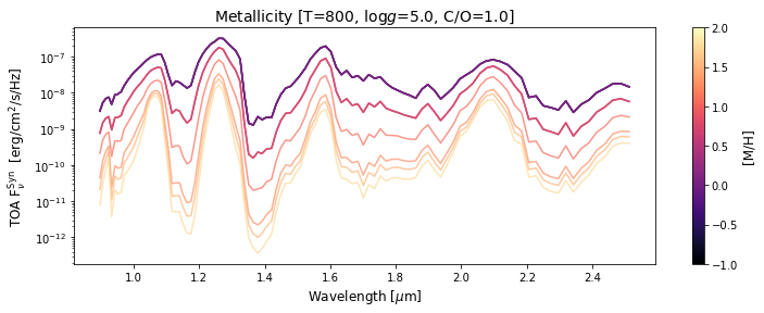
Plot the brown dwarf datasets for [M/H]= -1.0 - 2.0 while other paremeters are constnat (Teff=800, log g=5.0, C/O=1.0)
[10]:
# Define the filter bounds
filter_bounds = {'gravity': (5.,5),
                 'c_o_ratio' : (1.,1.),
                 'metallicity' : (-1,2),
                 'temperature': (800, 800)}


# Call the function to filter the dataset
plot_filtered_spectra(
                        dataset = train_BD,
                        filter_bounds = filter_bounds,
                        feature_to_plot = 'metallicity',
                        title_label = '[T='+str(filter_bounds['temperature'][0])+
                                ', log$g$='+str(filter_bounds['gravity'][0])+
                                ', C/O='+str(filter_bounds['c_o_ratio'][0])+']',
                        wl_synthetic = wavelength_values,
                        output_names = output_names,
                        __reference_data__ = __reference_data_path__,
                           __save_plots__=True,
                    )
